Risk management - Simple estimating of risk – more detail
Simple estimating of risk – more detail
Previously [see Simple estimating of risk], we had considered values for increases in duration should a risk materialise of:
| MAXIMUM: | 11 weeks |
| LIKELY: | 9 weeks (in between and considered the most probable) |
| MINIMUM: | 7 weeks |
This lead us to look at the ranges:
| MAXIMUM: | 10 to 12 weeks |
| LIKELY: | 8 to 10 weeks |
| MINIMUM: | 6 to 8 weeks |
We then came up with likelihoods of these ranges being the correct values:
| MINIMUM: | 20% or 0.2 chance of occurrence |
| MAXIMUM: | 30% or 0.3 chance of occurrence (slightly increased chance) |
| LIKELY: | 50% or 0.5 (i.e. 100% or 1.0 minus the sum of the others and the most likely) |
We could take this one step further to look at possible impact values higher and lower.
Step 1
| Impact | Original | step 1 |
|---|---|---|
| Likelihood | ||
| 3 | ||
| 5 | 0.1 | |
| 7 | 0.2 | 0.2 |
| 9 | 0.5 | 0.4 |
| 11 | 0.3 | 0.2 |
| 13 | 0.1 | |
| 15 | ||
We could take the accuracy one step further again.
Step 2
| Impact | Original | step 1 | step 2 |
|---|---|---|---|
| Likelihood | |||
| 3 | 0.05 | ||
| 5 | 0.1 | 0.10 | |
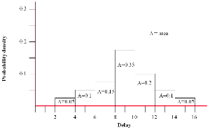
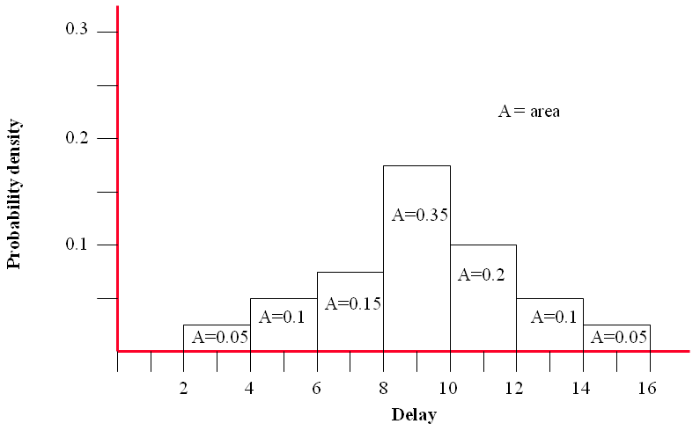
| 7 | 0.2 | 0.2 | 0.15 |
| 9 | 0.5 | 0.4 | 0.35 |
| 11 | 0.3 | 0.2 | 0.20 |
| 13 | 0.1 | 0.10 | |
| 15 | 0.05 | ||
Each column still totals to 1.0. Each step will be based upon additional consideration of the risk and possibly extra data.
The PROBABILITY DENSITY FUNCTION (PDF) for step 2 is shown in the above diagram.
As previously we can work out the expected delay based upon ‘conditional’ and ‘unconditional’ scenarios.
The likelihood of the risk occurring is still 20% or 0.2.
Unconditional
| Impact | Step 2 | Contribution |
|---|---|---|
| Likelihood | ||
| 3 | 0.05 | 3 x 0.05 = 0.15 |
| 5 | 0.10 | 5 x 0.1 = 0.5 |
| 7 | 0.15 | 7 x 0.15 = 1.05 |
| 9 | 0.35 | 9 x 0.35 = 3.15 |
| 11 | 0.20 | 11 x 0.2 = 2.2 |
| 13 | 0.10 | 13 x 0.1 = 1.3 |
| 15 | 0.05 | 15 x 0.05 = 0.75 |
Total unconditional expected delay = 9.1 weeks
Conditional
We know that this is:
Unconditional value x probability of the risk occurring = conditional value
9.1 X 0.2 = 1.82 weeks.
In this case seeking the increased accuracy has made little difference to the overall result but it may do depending on the considerations and additional data and information.
Again we can check the above by:
| Impact | Step 2 | Contribution |
|---|---|---|
| Likelihood | ||
| 0 | 0.8 | 0 x 0.8 = 0 |
| 3 | 0.05 | 3 x 0.05 x 0.2 = 0.03 |
| 5 | 0.10 | 5 x 0.1 x 0.2 = 0.10 |
| 7 | 0.15 | 7 x 0.15 x 0.2 = 0.21 |
| 9 | 0.35 | 9 x 0.35 x 0.2 = 0.63 |
| 11 | 0.20 | 11 x 0.2 x 0.2 = 0.44 |
| 13 | 0.10 | 13 x 0.1 x 0.2 = 0.26 |
| 15 | 0.05 | 15 x 0.05 x 0.2 = 0.15 |
Total conditional expected delay = 1.82 weeks
Why go to the higher accuracy of extra steps?
If you ask a person their opinion for the likely ranges in a simple case like this you will tend to get the simple view of:
| MAXIMUM: | 10 to 12 weeks |
| LIKELY: | 8 to 10 weeks |
| MINIMUM: | 6 to 8 weeks |
Thinking outside these confined limits may be narrow. The extra two steps forces people to refine their estimate by stretching the range of possibilities.
The only way to be more confident about a particular value is to collect data of actual experience over many projects which is unlikely.
The simple statistical approach shown is probably adequate for many people in many situations.
The use of more complex systems may have their individual merits but will not be examined in this basics package.
The PROBABILITY DENSITY FUNCTION (PDF) curves that we have seen are simple models requiring objective estimates of the expected values and their likelihoods.
It is a simple estimate from which we are able to calculate a ‘conditional’ and ‘unconditional’ delay should the risk occur.
The estimate will be based upon personal opinion backed up by other information and experience.
A common approach is to simplify it still further by using a ‘triangular distribution’. This involves keeping to a scenario where we have a an upper and lower limit with our best estimate in between.
It is assumed that the actual value will not lie outside of the upper and lower boundaries.
This would be:
| MAXIMUM: | 11 weeks |
| LIKELY: | 9 weeks (in between and considered the most probable) |
| MINIMUM: | 7 weeks |
It is then assumed that the distribution between the points is linear, forming a triangle.
For reasons described earlier the ‘triangular distribution’ may suffer from ‘narrowness’ of thought in terms of setting the upper and lower limits.
This system is referred to more explicitly in elsewhere [see PDF Simplified version].
Some problems encountered when trying to get subjective estimates are shown next [see Simple estimation problems].