Risk management - Simple branching
Simple branching
In the previous examples [see simple network, simple network no lag and simple network with lag] all activities are carried out.
We will now see what happens when there is a possible branch in the activity network.
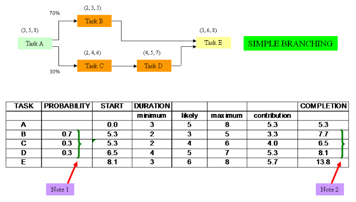
The above diagram shows 2 potential pathways.
The first has a 70% chance of occurring and is the PLANNED FOR pathway, this is what we expect to happen.
However, we need to be aware of a contingency that may occur which, from the above, must have a probability of 30%.
One or the other pathway will exist not both to get us to the start of task E.
In this case, tasks C and D represent the contingency plan. We hope task B is what will happen. There will be a trigger in the plan to activate tasks C and D.
These may need refining once the trigger is activated.
When would we need to allow for this?
It could happen on many occasions.
If, for example, there is a decision point after Task A then either pathway may be possible with Task B being more likely.
Another typical example would be for Quality Control testing where the differing pathways may represent reworking or fixing a problem before you can go on.
If the decision point is more of a strategic nature then the chosen pathway may be a completely different activity network and not meet up again with Task E for example.
That is the project changes fundamentally.
The above diagram represents a spreadsheet for a simple branching activity network where Task B and Task C begin at the same time but Task C is part of a contingency pathway.
The spreadsheet shows the following fields:
TaskLists the task activities as described in the network.
ProbabilityShows the probabilities of the task occurring.
StartThis is the start time of each task as calculated in the spreadsheet.
DurationThese are the 3 point estimates showing the MINIMUM, LIKELY and MAXIMUM.
ContributionThis is the average of the 3 point estimate values (MINIMUM + LIKELY + MAXIMUM)/3.
CompletionThis is the calculated end date or completion for each task. In the main this is the sum of the start value and the contribution, however, this is slightly more complex for activity networks where probabilities are taken into account, as here.
Note 1 and 2:
As referred to in the previous examples the contribution of each task is the sum of the minimum, likely and maximum values and divided by 3 to get the average.
In addition, we have to take into account the probabilities of the pathways involving Tasks B and C,D.
The contribution is calculated as normal.
The contribution is then multiplied by the probability and then added to the start duration to get to the completion duration.
For example, for Task B:
Start = 5.3 weeks
Contribution = 3.3 weeks
Probability = 0.7
Completion duration = (3.3 x 0.7) + 5.3 = 7.7 weeks (rounded up when calculated in the spreadsheet).
Note that the PROBABILITY for Task C and Task D is the same = 0.3.
The start values for both Task B and Task C are the same = 5.3.
The end of Task B is 7.7 weeks and Task D is 8.1 weeks so 8.1 weeks is taken as the start of Task E.
The final activity network completion date will be the end of Task E which is 8.1 + 5.7 (its 3 point estimate contribution) = 13.8.
Simulation
The spreadsheet simulation will carry out perhaps 300 to 1000 iterations and each time will firstly set Task A to a value based upon its 3 point estimate.
This will lead to a completion time for Task A which will be the start time of Tasks B and C. Each of these will in turn have a duration based upon their 3 point estimates affording individual completion dates. Eventually, there will be a value calculated for the completion date of Task D.
This final completion date will be recorded.
Over many iterations a MONTE CARLO distribution will result having a MINIMUM duration of (3 + 6 + 3) = 12 weeks and a MAXIMUM of (8 + 13 + 8) = 27 weeks.
The MINIMUM time is based upon the minima for Tasks C (2 weeks) and Task D (4 weeks), giving 6 weeks.
The MAXIMUM time is based upon the maxima for Tasks C (6 weeks) and Task D (7 weeks), giving 13 weeks.
From this data a graph of PROBABILTY versus TOTAL DURATION will be formed.
In a similar vein to the ‘cost’ scenario we will be able to, for example, set a ‘total duration’ at which there is a ‘likelihood’ of 20% of it being exceeded.
The TOTAL DURATION added on to the start date of 0.0 will give the project COMPLETION DATE.
In addition, CORRELATED EVENTS could be included as for the ‘cost risk assessment’. For this one would need to identify the INDEPENDENT task and then the DEPENDANT tasks which take their lead from it according to the underlying cause.
When looking at the spreadsheet and the mechanism for the iteration it is worth remembering that the probability values will not actually be seen as 0.7 or 0.3 (although the software might possibly be set to show this). This is because the software doesn’t actually provide a value of 0.7. In effect, it will give the pathway through Task B a value of ‘1’ or ‘0’ (ON or OFF).
When the value is ‘1’ the software will ignore the alternative pathway (which will be set to ‘0’) and set a value for Task B. This will lead to a calculation of the total duration for the completion of Task E.
In practice the software will set this pathway probability value to ‘1’ approximately 7 times in every 10 iterations, leading to a 70% chance of occurrence.
Naturally, the other pathway (through Task C) will be set in the opposite manner to get a 30% chance of occurrence.